Overview
By early 2018, I was just getting interested in investing. I was finally not living 100% paycheck-to-paycheck, and I had a coworker who was interested in talking about it. As someone trained in uncertainty, it irked me to read about 7% returns on average. I know the interpretation has to do with long-term averages (based on historical results), but the market is very volatile. So I set out to put something together that would more accurately capture market volatility. Specifically, I wanted to know how much better it would be to invest money in an index fund instead of moving it into a high-yield savings account with a 2% interest rate.
Spoiler: Yes, investing in an index fund has higher returns in the long run, but that assumes that previous market conditions are the norm and will continue.
Historical US Market Data
R Detail and Libraries
R.version.string
## [1] "R version 3.6.1 (2019-07-05)"
library(tidyverse)
## -- Attaching packages ------------------------- tidyverse 1.2.1 --
## v ggplot2 3.2.1     v purrr   0.3.2
## v tibble  2.1.3     v dplyr   0.8.3
## v tidyr   0.8.3     v stringr 1.4.0
## v readr   1.3.1     v forcats 0.4.0
## -- Conflicts ---------------------------- tidyverse_conflicts() --
## x dplyr::filter() masks stats::filter()
## x dplyr::lag()    masks stats::lag()
library(rvest)
## Loading required package: xml2
##
## Attaching package: 'rvest'
## The following object is masked from 'package:purrr':
##
##     pluck
## The following object is masked from 'package:readr':
##
##     guess_encoding

# Other Libraries used:
## scales
## forecast
Get S&P 500 Data
It was much harder to get market data than I expected. This website, https://www.thebalance.com/stock-market-returns-by-year-2388543, has yearly returns, and the S&P 500 is a decent index for the whole US Market. Web tables are fairly easy to work with in R, but sometimes, there’s a bit of trial-and-error involved with scraping the right table and formatting the resulting list.
website = "https://www.thebalance.com/stock-market-returns-by-year-2388543"

table_list = website %>%
  read_html() %>%
  html_nodes("table") %>%
  html_table(header = TRUE)

sp_500 = tibble(years = as.numeric(table_list[[1]][-1,1]),
                returns = as.numeric(table_list[[1]][-1,2])/100)

dim(sp_500)
## [1] 31  2

head(sp_500)
## # A tibble: 6 x 2
##   years returns
##   <dbl>   <dbl>
## 1  1986   0.185
## 2  1987   0.052
## 3  1988   0.168
## 4  1989   0.315
## 5  1990  -0.031
## 6  1991   0.305
Examine S&P 500 Data
ggplot(data = sp_500) +
  geom_histogram(aes(returns), bins = 10, col = 'forestgreen') +
  scale_x_continuous(labels = scales::percent)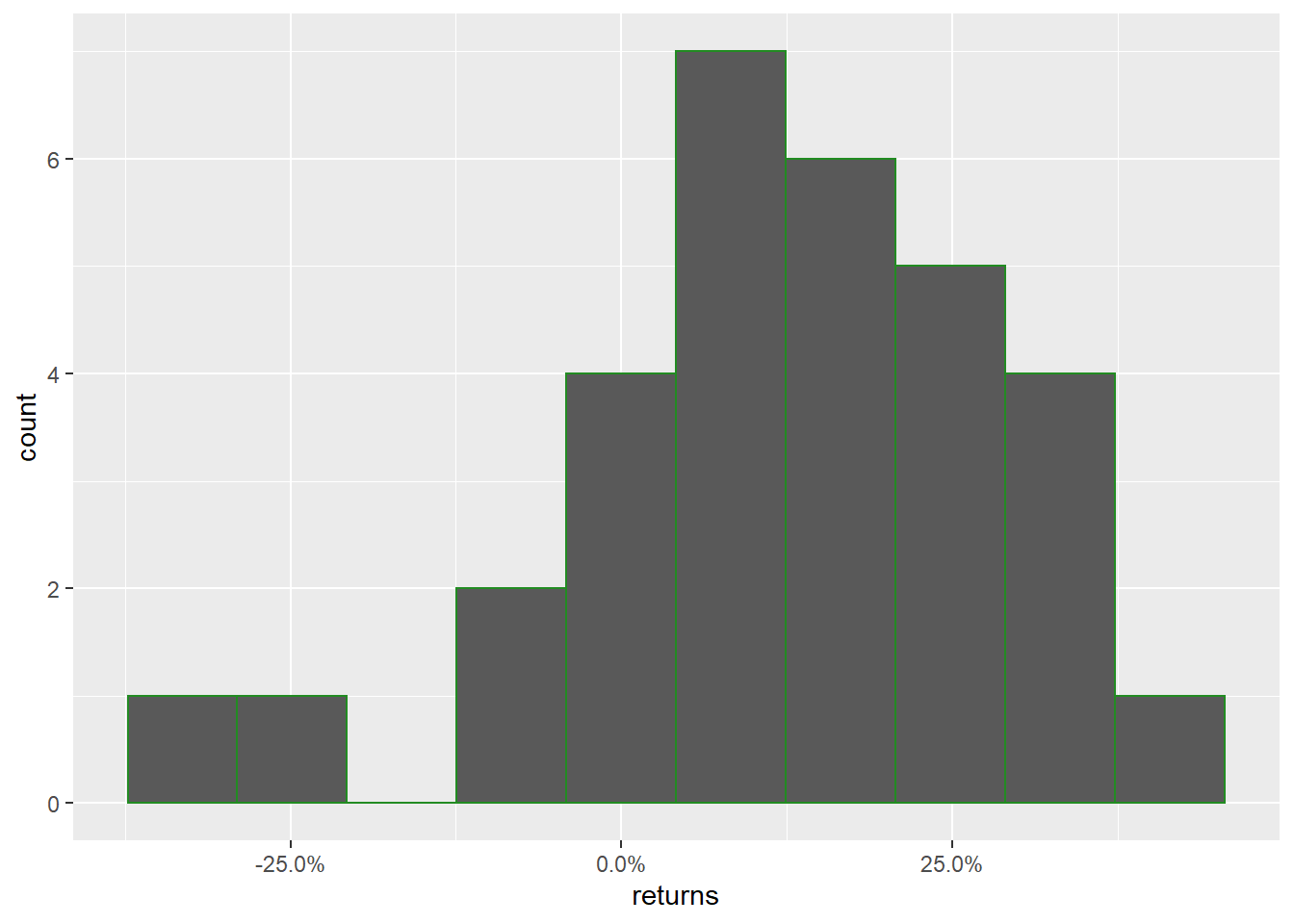
Hmm, so this is definitely not a nice uniform (flat) or normal distribution of yearly returns.
ggplot(data = sp_500, aes(x=years, y = returns)) +
  geom_line() +
  geom_point() +
  geom_hline(yintercept = 0, linetype = 'dashed') +
  labs(title = "S&P 500 Yearly Returns") +
  scale_y_continuous(labels = scales::percent)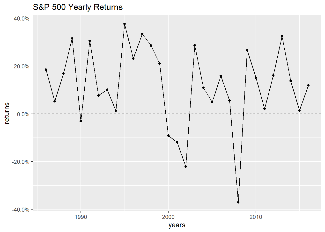
It kind of bounces all over the place, but there have been a lot of good years. It doesn’t look like consecutive years are highly correlated, but it never hurts to look at some auto-correlation plots. (Note: Base R includes the acf function, but I prefer the one in the forecast package because it excludes lag 0.)
par(mfrow = c(1,2))

forecast::Acf(sp_500$returns)
## Registered S3 method overwritten by 'xts':
##   method     from
##   as.zoo.xts zoo
## Registered S3 method overwritten by 'quantmod':
##   method            from
##   as.zoo.data.frame zoo
## Registered S3 methods overwritten by 'forecast':
##   method             from
##   fitted.fracdiff    fracdiff
##   residuals.fracdiff fracdiff
forecast::Pacf(sp_500$returns)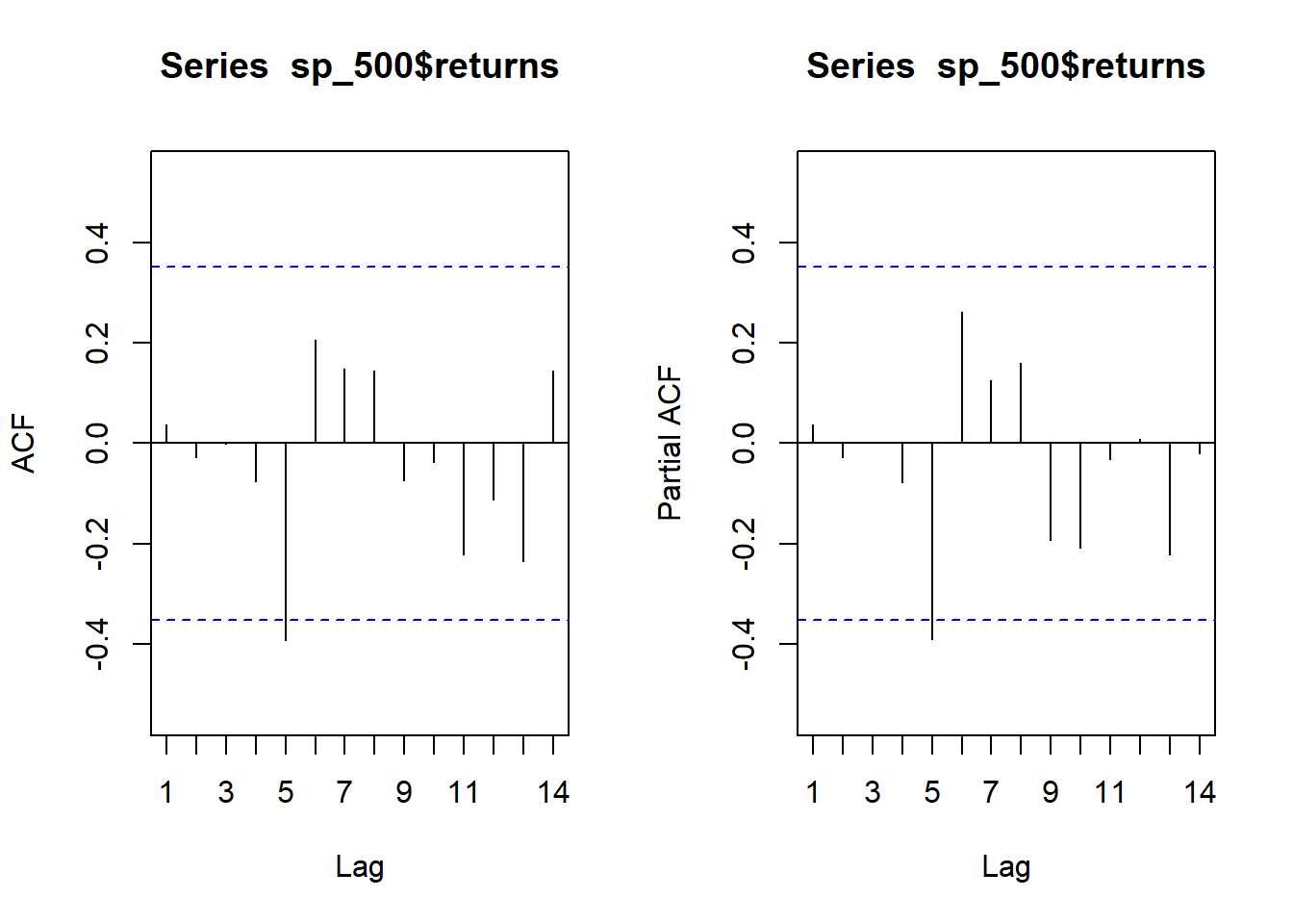
# reset the plotting space to a 1x1 grid
par(mfrow = c(1,1))
Looks good here; we aren’t seeing large correlations at early lags. While both show a significant correlation at lag = 5, it’s fairly safe to ignore that and let some young, econometric students dive into it.
So what numbers are we actually working with:
summary(sp_500$returns)
##    Min. 1st Qu.  Median    Mean 3rd Qu.    Max.
## -0.3700  0.0350  0.1370  0.1184  0.2480  0.3760
Simulation
We want to use the data in some way that our future-looking yearly results are a series of random simulations. Assuming a standard percentage will repeat itself every year is useful when speaking generally, but it is not as informative when making random simulations. In other words, if we use a single value, such as the commonly seen 7% or our average value 11.8%, we will not have any possibility of getting extreme values.
Should you smooth the yearly returns?
We’ve seen how the market returns are distributed in the histogram above, and we’ve seen the summary statistics. Sometimes, if you have extreme values in your dataset you might want to exclude them or limit their influence. You can do this by smoothing. Let’s investigate smoothing to see how it affects our distribution of yearly returns.
smoothed_sample = function(x,smoothing){
  sum(sample(x, size = smoothing, replace = TRUE))/smoothing
}
Here’s a smoothing function that samples (with replacement) a vector and averages the sample. It’s basically how you bootstrap a mean; however, I want it to be flexible so I can see the difference between smoothing parameters. My goal is to not over-smooth the results.
Now I’ll call my function a bunch of times and look at how the distribution changes. Note that Smoothing Parameter = 1 is ‘no smoothing’ because it is drawing samples of size 1.
par(mfrow = c(3,3))
for(i in 1:9){

  smoothed_returns = replicate(1000,smoothed_sample(sp_500$returns, i))

  hist(smoothed_returns, main = paste("Smoothing Parameter =",i), xlim = c(-.4,.4))
}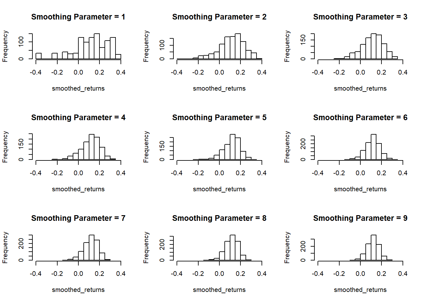
# reset the plotting space to a 1x1 grid
par(mfrow = c(1,1))
So as the smoothing parameter gets larger (the size of the sample to be averaged), we see the histograms converging on the mean of our dataset 11.8%. Even with a smoothing parameter of 2, we lose our extreme values, so I don’t think this dataset is a good candidate for smoothing.
Initialize Variables
These are the initial inputs we’ll need to calculate savings account returns, and we’ll go ahead and set up the market returns vector.
The principle is our starting amount ($5,000), and we’ll plan to contribute $200 each month. As of this time, some online savings accounts offer yearly interest rates over 2%, but don’t take that as a complete given. Interest rates fluctuate, but not as much as the stock market. We’ll look at the simulation over the course of 30 years, and run 500 market simulations. (I think too many simulations leads to graphs looking overly smooth, and they can wash out the individual simulations.)
principle = 5000
monthly_contribution = 200
savings_interest = .021
pred_years = 30
how_many_simulations = 500

market_vector = NULL
savings_vector = NULL

market_vector[1] = principle
savings_vector[1] = principle
Calculate Savings Account
Because we are going to make monthly contributions, there’s no need to use the equation for compound interest. Instead we’ll just calculate each month. Then, we’ll take our monthly results, and store the ‘January’ months in a dataframe.
This analysis assumes that interest is compounded monthly, but it’s more likely that your savings account interest is compounded daily.
for(i in 2:(pred_years*12)){
  savings_vector[i] = (savings_vector[i-1] + monthly_contribution)*(1 + savings_interest/12)
}

year_mon_index = 12 * (1:pred_years) - 11

year_mon_index
##  [1]   1  13  25  37  49  61  73  85  97 109 121 133 145 157 169 181 193
## [18] 205 217 229 241 253 265 277 289 301 313 325 337 349

savings = tibble(year = 1:pred_years,
                 savings_amount = round(savings_vector[year_mon_index],0))

tail(savings)
## # A tibble: 6 x 2
##    year savings_amount
##   <int>          <dbl>
## 1    25          83215
## 2    26          87407
## 3    27          91688
## 4    28          96060
## 5    29         100524
## 6    30         105083
Run Market Simulations
Instead of using the fixed savings_interest, we’ll take a random sample from the market returns for each year. There’s a bit of disconnect here because we are assuming that this interest is compounded yearly… but at the end of the day, it’s really not that big of a difference.
(You’ll have to take my word for it, but I don’t think it’s a good idea to add in an error term, \(\varepsilon \sim N(0,\sigma)\), to our simulation. Once again, I find that it over-smooths the results. Perhaps adding in an error term would be useful if you were doing more formal, hierarchical modeling and could find a nice small standard deviation for \(\varepsilon \sim N(0,\sigma)\).)
random_investing = tibble(simulation = as.factor(sort(rep(1:how_many_simulations,pred_years))),
                          year = rep(1:pred_years,how_many_simulations),
                          value = 0)


for(j in 1:how_many_simulations){
  for (i in 2:pred_years){
    market_vector[i] = (market_vector[i-1] + monthly_contribution*12)*(1+ sample(sp_500$returns, 1))
  }

  random_investing[random_investing$simulation==j,3] = market_vector
}

head(random_investing)
## # A tibble: 6 x 3
##   simulation  year  value
##   <fct>      <int>  <dbl>
## 1 1              1  5000
## 2 1              2  9872.
## 3 1              3 16137.
## 4 1              4 17963.
## 5 1              5 24639.
## 6 1              6 17034.
Plot Results
Now, let’s plot the results of our simulations and savings account.
ggplot(data = random_investing, aes(x = year, y = value)) +
  geom_line(aes(group = simulation, color = "Market \nSimulation")) +
  stat_summary(fun.y = "median", geom = "line", aes(color = "Simulation \nMedian"), size = 1.1)+
  geom_line(data = savings, aes(x = year, y = savings_amount, color = "Savings"), size = 1.5) +
  labs(title = "Simulated Account Balance", y = "Account Value") +
  scale_y_continuous(labels = function(l){ trans = l/1000; paste0(trans,"K")}) +
  scale_color_manual("", values = c("Savings" = "red",
                                        "Market \nSimulation" = "black",
                                        "Simulation \nMedian" = "blue"))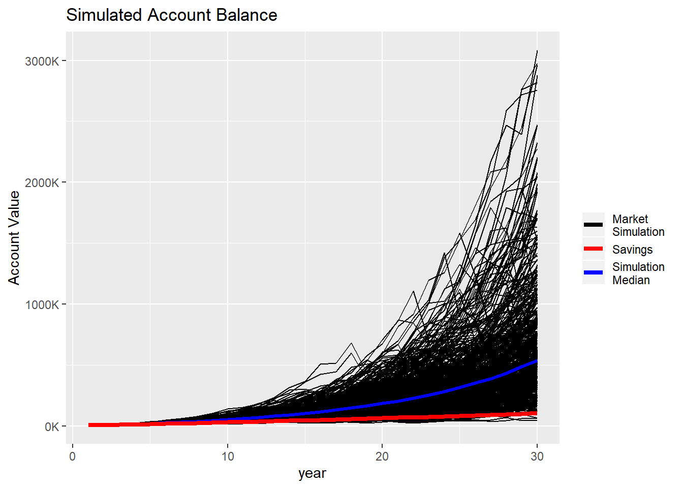
Conclusion
So, yes, investing in an index fund has higher returns in the long run, but that assumes that previous market conditions are the norm and will continue. It is interesting that there are some scenarios below the savings line, and there are only a few extremely high values.