Overview
The Last Digit of Total Points is a game of chance relating to the final score of a sporting event. In this post, I’m going to discuss how you would play the Last Digit game for an NFL game, namely, The Super Bowl. The beauty of this game is that you don’t actually have to know anything about football or anything about the particular game to have a decent shot at winning. To win, you need to guess the last digit of the sum of final scores.
For example, if the final score of a game is 27-24, then you add the scores together to get 51. Thus, the winning last digit is 1. So really, you just have to pick a number between 0 and 9. Some simple analysis should tell us which numbers appear most frequently, but it would be painful to go through this process manually.
Instead of doing this manually, we’ll leverage R, the Tidyverse, rvest, and ESPN.
Historical Analysis
R Detail and Libraries
R.version.string
## [1] "R version 3.5.3 (2019-03-11)"
library(rvest)
## Loading required package: xml2
library(tidyverse)
## -- Attaching packages --------------------------- tidyverse 1.2.1 --
## v ggplot2 3.1.1       v purrr   0.3.2
## v tibble  2.1.1       v dplyr   0.8.0.1
## v tidyr   0.8.3       v stringr 1.4.0
## v readr   1.3.1       v forcats 0.4.0
## -- Conflicts ------------------------------ tidyverse_conflicts() --
## x dplyr::filter()         masks stats::filter()
## x readr::guess_encoding() masks rvest::guess_encoding()
## x dplyr::lag()            masks stats::lag()
## x purrr::pluck()          masks rvest::pluck()
library(knitr)
library(kableExtra)
##
## Attaching package: 'kableExtra'
## The following object is masked from 'package:dplyr':
##
##     group_rows
NFL Scores Data
I found that the NFL schedule webpage on ESPN was easier to work with than the NFL scores webpage. rvest is the easiest to work with when you have a simple html table, but I didn’t want to spend a bunch of time searching for a simple table of NFL scores.
The downside of using ESPN’s website is that it has the schedule broken out by-week. With a little bit of playing around, you can see that URLs with this form get you what you want: http://www.espn.com/nfl/schedule?week=16&year=2017&seasontype=2.
Now, to get all of the scores, we just need to loop through the weeks and years. (Leave seasontype=2. It looks like 1 is the only other option, and seasontype=1 just overrides your other parameters and brings you to the current schedule.)
I know the R junkies out there will not be pleased that I’m writing for-loops in R, and yes, there is probably a way for me to vectorize my code to accomplish the same thing. But this is easier for me to think about and create.
Vector of URL’s
current_season = 2018
num_seasons = 4

website = matrix(NA, nrow = 17, ncol = num_seasons)

for (j in 1:num_seasons){
  for (i in 1:17){

    year = 2018 - num_seasons + j

    website[i,j] = paste0("http://www.espn.com/nfl/schedule?week=",i,"&year=",year,"&seasontype=2")
  }
}

website_vector = as.vector(website)
length(website_vector)
## [1] 68

head(website_vector)
## [1] "http://www.espn.com/nfl/schedule?week=1&year=2015&seasontype=2"
## [2] "http://www.espn.com/nfl/schedule?week=2&year=2015&seasontype=2"
## [3] "http://www.espn.com/nfl/schedule?week=3&year=2015&seasontype=2"
## [4] "http://www.espn.com/nfl/schedule?week=4&year=2015&seasontype=2"
## [5] "http://www.espn.com/nfl/schedule?week=5&year=2015&seasontype=2"
## [6] "http://www.espn.com/nfl/schedule?week=6&year=2015&seasontype=2"
# .
# .
# .
tail(website_vector)
## [1] "http://www.espn.com/nfl/schedule?week=12&year=2018&seasontype=2"
## [2] "http://www.espn.com/nfl/schedule?week=13&year=2018&seasontype=2"
## [3] "http://www.espn.com/nfl/schedule?week=14&year=2018&seasontype=2"
## [4] "http://www.espn.com/nfl/schedule?week=15&year=2018&seasontype=2"
## [5] "http://www.espn.com/nfl/schedule?week=16&year=2018&seasontype=2"
## [6] "http://www.espn.com/nfl/schedule?week=17&year=2018&seasontype=2"
Create Vector of Results
rvest works by looking at the html code of a website, finding a defined tag, and storing something in a list. So in this code chuck, I create an empty variable and fill it as a list of dataframes. Then, I extract the results from each of those dataframes as a string vector.
totals_list = NULL

for (i in 1:length(website_vector)){

  temp_list = website_vector[i] %>%
    read_html() %>%
    html_nodes("table") %>%
    html_table(header = TRUE, fill = TRUE)

  totals_list = append(totals_list, temp_list)

  rm(temp_list)

}

# How long is this list?
length(totals_list)
## [1] 235

# What does each dataframe in the list look like?
names(totals_list[[1]])
## [1] "matchup"          ""                 "result"
## [4] "passing leader"   "rushing leader"   "receiving leader"
## [7] NA


results = NULL

for (i in 1:length(totals_list)) {
  results = c(results,totals_list[[i]]$result)

}

head(results)
## [1] "NE 28, PIT 21"       "BUF 27, IND 14"      "GB 31, CHI 23"
## [4] "STL 34, SEA 31 (OT)" "NYJ 31, CLE 10"      "MIA 17, WSH 10"
Turn Results Vector into Dataframe
# Remove commas "," using gsub
# Split the results vector into a matrix along each space " "
games_matrix = str_split(gsub(",","",results), " ", simplify = T)

# Name the columns
colnames(games_matrix) = c("away", "away_score", "home", "home_score", "overtime")

# Turn the matrix into a tibble
# Make sure numbers are numbers
# Add some calculations
# There was one game that was postponed
games_df  = as.tibble(games_matrix) %>%
  mutate(away_score = as.numeric(away_score),
         home_score = as.numeric(home_score),
         score_total = `away_score`+ `home_score`,
         final_number = (str_sub(score_total, -1,-1)),
         tie_game = if_else(away_score == home_score, "tie", "no tie")) %>%
  filter(away != "Postponed") %>%
  mutate(season = sort(rep(((current_season-num_seasons+1):current_season),256)))
## Warning: `as.tibble()` is deprecated, use `as_tibble()` (but mind the new semantics).
## This warning is displayed once per session.

games_df
## # A tibble: 1,024 x 9
##    away  away_score home  home_score overtime score_total final_number
##    <chr>      <dbl> <chr>      <dbl> <chr>          <dbl> <chr>
##  1 NE            28 PIT           21 ""                49 9
##  2 BUF           27 IND           14 ""                41 1
##  3 GB            31 CHI           23 ""                54 4
##  4 STL           34 SEA           31 (OT)              65 5
##  5 NYJ           31 CLE           10 ""                41 1
##  6 MIA           17 WSH           10 ""                27 7
##  7 CAR           20 JAX            9 ""                29 9
##  8 KC            27 HOU           20 ""                47 7
##  9 ARI           31 NO            19 ""                50 0
## 10 SD            33 DET           28 ""                61 1
## # ... with 1,014 more rows, and 2 more variables: tie_game <chr>,
## #   season <int>
Make some graphs
ggplot(data = games_df, aes(x = final_number, fill = as.factor(season)))+
  geom_bar(aes(y = ..count.., group =as.factor(season))) +
  facet_wrap(~season, ncol = 2) +
  labs(y = "Count", fill = "Season", title = "Count By Season")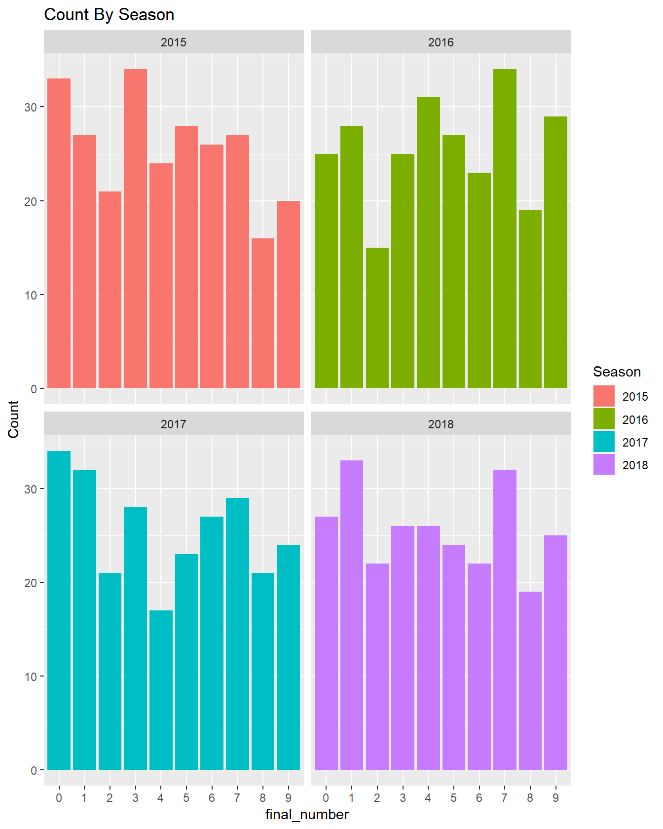
ggplot(data = games_df, aes(x = final_number, fill = as.factor(season)))+
  geom_bar(aes(y = ..prop.., group =as.factor(season))) +
  facet_wrap(~season, ncol = 2) +
  labs(y = "Percent", fill = "Season", title = "Percent By Season")+
  scale_y_continuous(labels = scales::percent)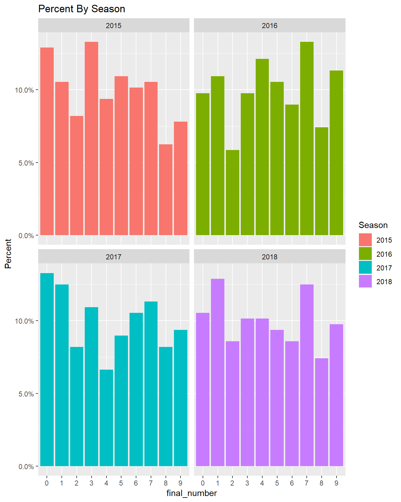
ggplot(data = games_df, aes(x = final_number))+
  geom_bar(stat= "count", fill = "darkgreen") +
  labs(y = "Count", title = paste0("Count for All Seasons (",(current_season-num_seasons+1),"-",current_season, ")"))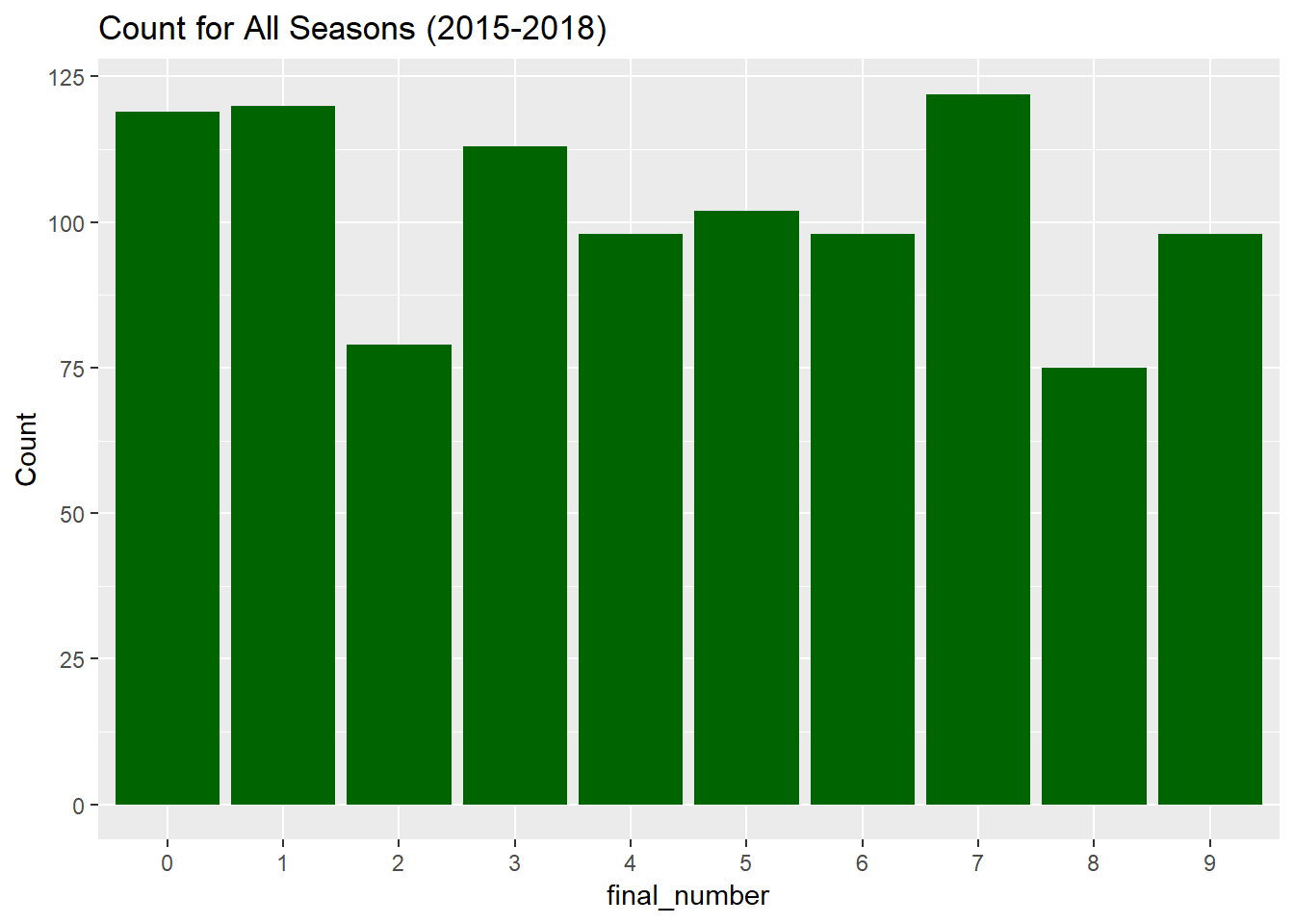
ggplot(data = games_df, aes(x = final_number))+
  geom_bar(aes(y = ..prop.., group = 1), stat = "count" , fill = "darkgreen") +
  labs(y = "Percent", title = paste0("Percent for All Seasons (",(current_season-num_seasons+1),"-",current_season, ")"))+
  scale_y_continuous(labels = scales::percent)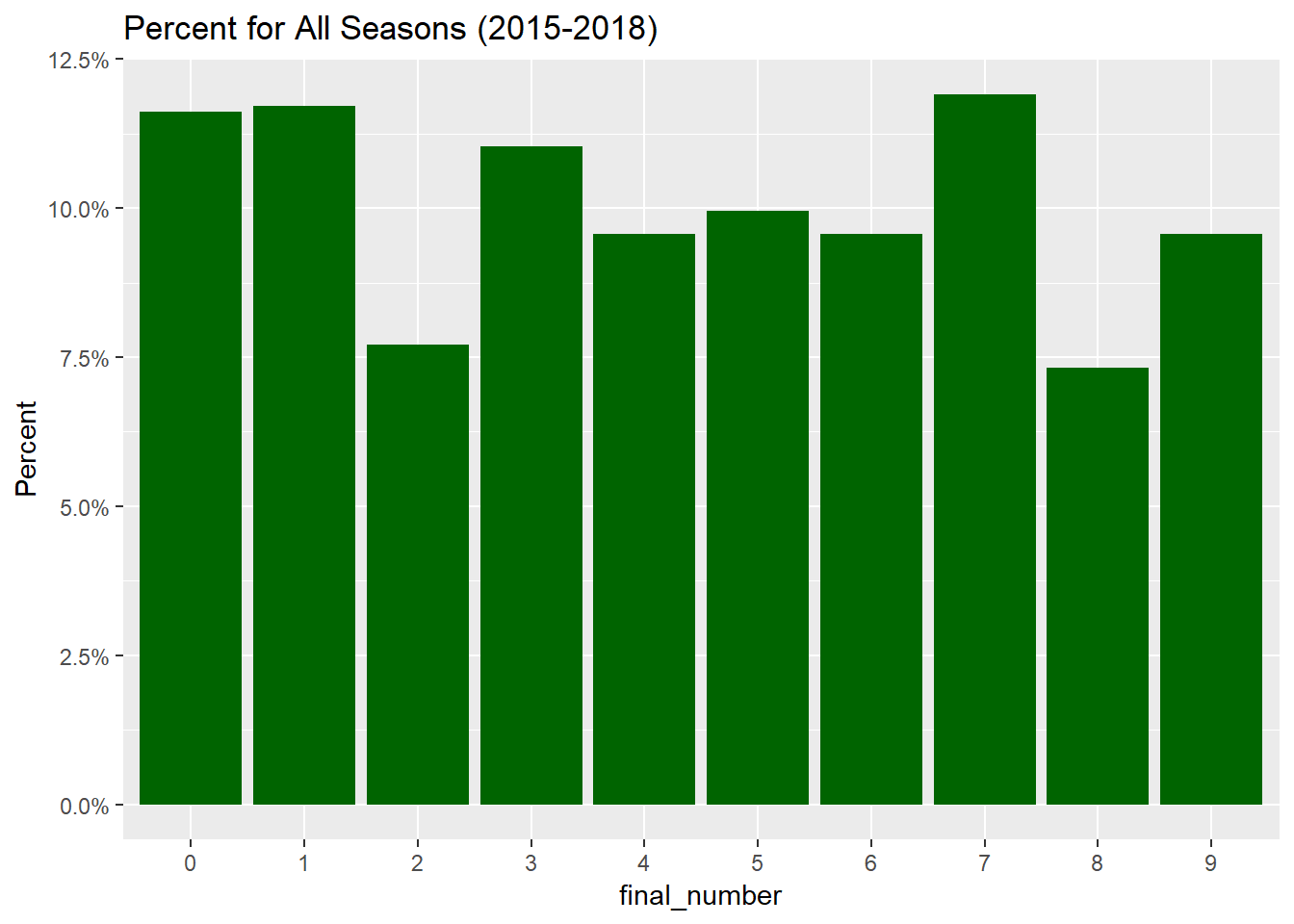
# Leverage the kable function to print a nice table for overallMake a nice table of overall results
summarized_table = games_df %>%
        group_by(final_number) %>%
        summarize(count = n()) %>%
        mutate(percentage = scales::percent(count/sum(count)))

kable(summarized_table,  align = 'c') %>%
  kable_styling("striped", full_width = FALSE) %>%
add_header_above(c("Overall Tabular Results" = 3))| final_number | count | percentage |
|---|---|---|
| 0 | 119 | 11.62% |
| 1 | 120 | 11.72% |
| 2 | 79 | 7.71% |
| 3 | 113 | 11.04% |
| 4 | 98 | 9.57% |
| 5 | 102 | 9.96% |
| 6 | 98 | 9.57% |
| 7 | 122 | 11.91% |
| 8 | 75 | 7.32% |
| 9 | 98 | 9.57% |
kable(arrange(summarized_table, desc(count)),  align = 'c') %>%
  kable_styling("striped", full_width = FALSE) %>%
add_header_above(c("Sorted Overall Tabular Results" = 3))| final_number | count | percentage |
|---|---|---|
| 7 | 122 | 11.91% |
| 1 | 120 | 11.72% |
| 0 | 119 | 11.62% |
| 3 | 113 | 11.04% |
| 5 | 102 | 9.96% |
| 4 | 98 | 9.57% |
| 6 | 98 | 9.57% |
| 9 | 98 | 9.57% |
| 2 | 79 | 7.71% |
| 8 | 75 | 7.32% |
Takeaways
The overall results are not seen in each season, so I’m not sure exactly what to make of this. I think your best bet is to go in the overall percentage order. If that doesn’t quite do it for you, then pick a score and do the math to see what the final number is.
I like Patriots beating the Rams 27 - 24, so I’m sticking with 1.