Intro
This post is a copy of the tensorflow.org ‘Regression: predict fuel efficiency’ tutorial https://www.tensorflow.org/tutorials/keras/basic_regression, but written in the R language using the tidyverse instead of python. It assumes that you have already downloaded Anaconda and have R connected to python.
Load Libraries and Verify Python
library(tidyverse)
## -- Attaching packages ---------------------------------------------------------------------- tidyverse 1.2.1 --
## v ggplot2 3.2.1     v purrr   0.3.2
## v tibble  2.1.3     v dplyr   0.8.3
## v tidyr   0.8.3     v stringr 1.4.0
## v readr   1.3.1     v forcats 0.4.0
## -- Conflicts ------------------------------------------------------------------------- tidyverse_conflicts() --
## x dplyr::filter() masks stats::filter()
## x dplyr::lag()    masks stats::lag()
library(lubridate)
##
## Attaching package: 'lubridate'
## The following object is masked from 'package:base':
##
##     date
library(rsample)
library(tensorflow)
library(keras)
library(recipes)
##
## Attaching package: 'recipes'
## The following object is masked from 'package:stringr':
##
##     fixed
## The following object is masked from 'package:stats':
##
##     step
library(yardstick)
## For binary classification, the first factor level is assumed to be the event.
## Set the global option `yardstick.event_first` to `FALSE` to change this.
##
## Attaching package: 'yardstick'
## The following object is masked from 'package:keras':
##
##     get_weights
## The following object is masked from 'package:readr':
##
##     spec
options(yardstick.event_first = FALSE)
reticulate::py_config()
## python: C:\PROGRA~3\ANACON~1\python.exe
## libpython: C:/PROGRA~3/ANACON~1/python37.dll
## pythonhome: C:\PROGRA~3\ANACON~1
## version: 3.7.3 (default, Mar 27 2019, 17:13:21) [MSC v.1915 64 bit (AMD64)]
## Architecture: 64bit
## numpy: C:\PROGRA~3\ANACON~1\lib\site-packages\numpy
## numpy_version: 1.16.2
## tensorflow: C:\PROGRA~3\ANACON~1\lib\site-packages\tensorflow\__init__.p
##
## python versions found:
## C:\PROGRA~3\ANACON~1\python.exe
## C:\ProgramData\Anaconda3\python.exeData
The Auto MPG dataset is available from the UCI Machine Learning Repository.
Download the data
dataset_path = get_file("auto-mpg.data",
                        "http://archive.ics.uci.edu/ml/machine-learning-databases/auto-mpg/auto-mpg.data")
Set column names
column_names = c('MPG','Cylinders','Displacement','Horsepower','Weight',
                'Acceleration', 'Model Year', 'Origin')
Import the data
auto_mpg = read_delim(file = dataset_path,
                      col_names = column_names,
                      delim = " ",
                      comment = "\t",
                      trim_ws = TRUE,
                      na = "?")
## Parsed with column specification:
## cols(
##   MPG = col_double(),
##   Cylinders = col_double(),
##   Displacement = col_double(),
##   Horsepower = col_double(),
##   Weight = col_double(),
##   Acceleration = col_double(),
##   `Model Year` = col_double(),
##   Origin = col_double()
## )

head(auto_mpg)
## # A tibble: 6 x 8
##     MPG Cylinders Displacement Horsepower Weight Acceleration `Model Year`
##   <dbl>     <dbl>        <dbl>      <dbl>  <dbl>        <dbl>        <dbl>
## 1    18         8          307        130   3504         12             70
## 2    15         8          350        165   3693         11.5           70
## 3    18         8          318        150   3436         11             70
## 4    16         8          304        150   3433         12             70
## 5    17         8          302        140   3449         10.5           70
## 6    15         8          429        198   4341         10             70
## # ... with 1 more variable: Origin <dbl>
Transform the data
We want to get rid of any rows containing NA, and we want to transform our Origin categorical column to multiple 1/0 indicator columns. For a slightly different, but ultimately equal analysis, you could encode the Origin column as a factor. (That would lead to other changes downstream in this workflow.)
dataset = auto_mpg %>%
  drop_na() %>%
  mutate("USA" = if_else(Origin == 1,1,0),
         "Europe" = if_else(Origin == 2,1,0),
         "Japan" = if_else(Origin == 3,1,0)) %>%
  select(-Origin)

# Alternative
# dataset$Origin = factor(dataset$Origin, labels = c("USA", "Europe", "Japan"))
Data Prep
Split dataset into testing and training
The rsample package contains a nice way to split your data into testing and training sets.
data_split <- initial_split(dataset, prop = 4/5, strata = NULL)
training_data <- training(data_split)
testing_data <- testing(data_split)
Examine Training Data
In order to mimic the Keras tutorial, we need to make a new function for displaying histograms, and then call it from the pairs function on the diagonal.
Additionally, we can see the summary data by calling the `summary function, and t just transposes it for slightly easier reading. The only thing summary doesn’t include is standard deviation, so we’ll utilize map to call the sd function for each column. map_dbl simplifies the output to a numeric vector instead of a list.
# Histogram in panel function copied from the hist help file.
panel.hist <- function(x, ...)
{
  usr <- par("usr"); on.exit(par(usr))
  par(usr = c(usr[1:2], 0, 1.5) )
  h <- hist(x, plot = FALSE)
  breaks <- h$breaks; nB <- length(breaks)
  y <- h$counts; y <- y/max(y)
  rect(breaks[-nB], 0, breaks[-1], y, col = "cyan", ...)
}

pairs(training_data %>%
        select(-USA, -Europe, -Japan),
      diag.panel = panel.hist)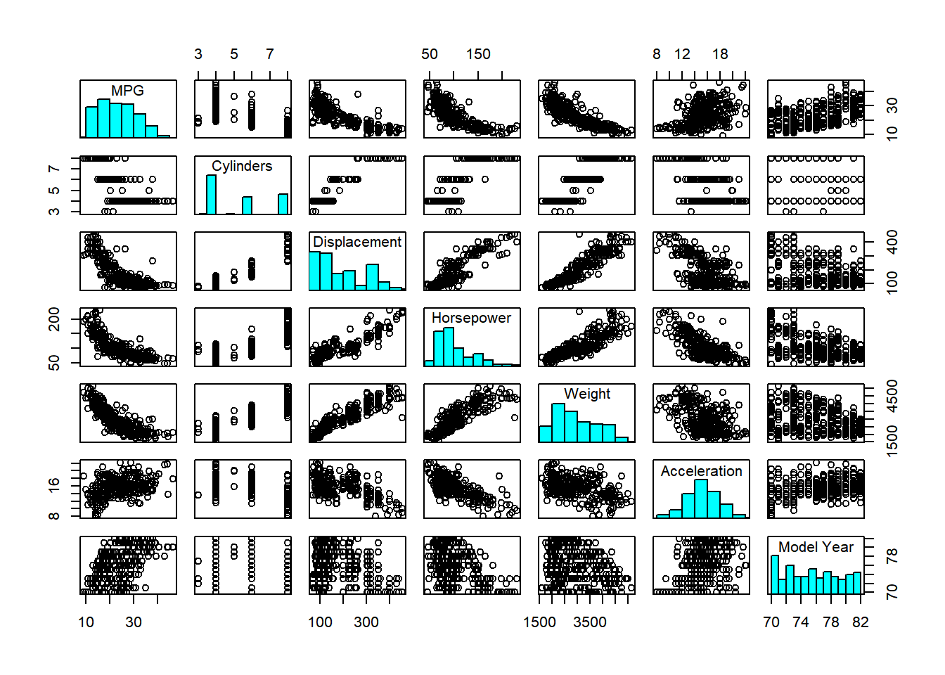
t(summary(training_data, digits = 2))
##
##      MPG      Min.   : 9     1st Qu.:18     Median :23     Mean   :24
##   Cylinders   Min.   :3.0    1st Qu.:4.0    Median :4.0    Mean   :5.5
##  Displacement Min.   : 68    1st Qu.:100    Median :151    Mean   :193
##   Horsepower  Min.   : 46    1st Qu.: 75    Median : 92    Mean   :104
##     Weight    Min.   :1613   1st Qu.:2219   Median :2790   Mean   :2963
##  Acceleration Min.   : 8     1st Qu.:14     Median :16     Mean   :15
##   Model Year  Min.   :70     1st Qu.:73     Median :76     Mean   :76
##      USA      Min.   :0.00   1st Qu.:0.00   Median :1.00   Mean   :0.64
##     Europe    Min.   :0.00   1st Qu.:0.00   Median :0.00   Mean   :0.16
##     Japan     Min.   :0.00   1st Qu.:0.00   Median :0.00   Mean   :0.21
##
##      MPG      3rd Qu.:29     Max.   :47
##   Cylinders   3rd Qu.:8.0    Max.   :8.0
##  Displacement 3rd Qu.:262    Max.   :455
##   Horsepower  3rd Qu.:125    Max.   :230
##     Weight    3rd Qu.:3612   Max.   :5140
##  Acceleration 3rd Qu.:17     Max.   :22
##   Model Year  3rd Qu.:79     Max.   :82
##      USA      3rd Qu.:1.00   Max.   :1.00
##     Europe    3rd Qu.:0.00   Max.   :1.00
##     Japan     3rd Qu.:0.00   Max.   :1.00

map_dbl(training_data, sd)
##          MPG    Cylinders Displacement   Horsepower       Weight
##    7.7877178    1.6922525  103.5508244   38.0154433  844.9186366
## Acceleration   Model Year          USA       Europe        Japan
##    2.5760046    3.7338775    0.4816487    0.3634829    0.4058068
Create recipe for standardizing predictors
The recipes package aims to make design matrix manipulation easy and repeatable. Just make sure you run prep() at the end!
rec = recipe(MPG ~ ., data = training_data) %>%
  step_center(all_predictors()) %>%
  step_scale(all_predictors()) %>%
  prep()

#bake(rec, testing_data, composition = "matrix")
The Keras Model
Build the model
From the tensorflow tutorial:
Let’s build our model. Here, we’ll use a Sequential model with two densely connected hidden layers, and an output layer that returns a single, continuous value. The model building steps are wrapped in a function, build_model, since we’ll create a second model, later on.
build_model = function(){

model = keras_model_sequential() %>%
  layer_dense(units = 64, activation = "relu", input_shape = ncol(training_data)-1) %>%
  layer_dense(units = 64, activation = "relu") %>%
  layer_dense(units = 1)

model %>%
  compile(loss = "mse",
          optimizer = "rmsprop",
          metrics = list("mae","mse"))

return(model)
}


model1 = build_model()

summary(model1)
## Model: "sequential"
## ___________________________________________________________________________
## Layer (type)                     Output Shape                  Param #
## ===========================================================================
## dense (Dense)                    (None, 64)                    640
## ___________________________________________________________________________
## dense_1 (Dense)                  (None, 64)                    4160
## ___________________________________________________________________________
## dense_2 (Dense)                  (None, 1)                     65
## ===========================================================================
## Total params: 4,865
## Trainable params: 4,865
## Non-trainable params: 0
## ___________________________________________________________________________
Set inputs and outputs
Use the recipe we defined earlier (rec) to bake (i.e. setup) the training data. Define x, the predictors, and y, the response variable.
training_baked = bake(rec, training_data, composition = "matrix")
x = subset(training_baked, select = -MPG)
y = training_baked[,"MPG"]
Fit the model
history1 = model1 %>% fit(
  x = x,
  y = y,
  batch_size = 50,
  epoch = 100
)

plot(history1)+
  labs(title = "Neural Net Metrics")+
  theme(strip.placement = "outside",
        strip.text.y = element_text(size = 9),
        plot.title = element_text(hjust = 0.5))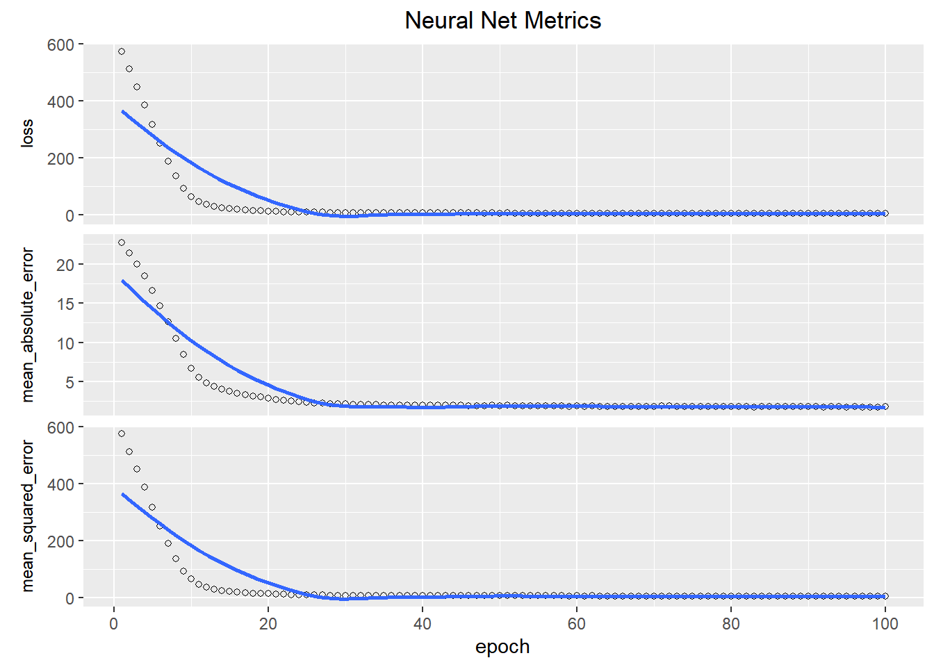
We can see that after a while, the model stopped getting better. We can add in a callback to stop it fitting more epochs.
We’ll use an EarlyStopping callback that tests a training condition for every epoch. If a set amount of epochs elapses without showing improvement, then automatically stop the training. [Note,] the patience parameter is the amount of epochs to check for improvement.
Refit the model
model2 = build_model()

history2 = model2 %>% fit(
  x = x,
  y = y,
  batch_size = 50,
  epoch = 100,
  callbacks = callback_early_stopping(monitor = "mean_squared_error", patience = 5)
)

plot(history2)+
  labs(title = "Neural Net Metrics")+
  theme(strip.placement = "outside",
        strip.text.y = element_text(size = 9),
        plot.title = element_text(hjust = 0.5))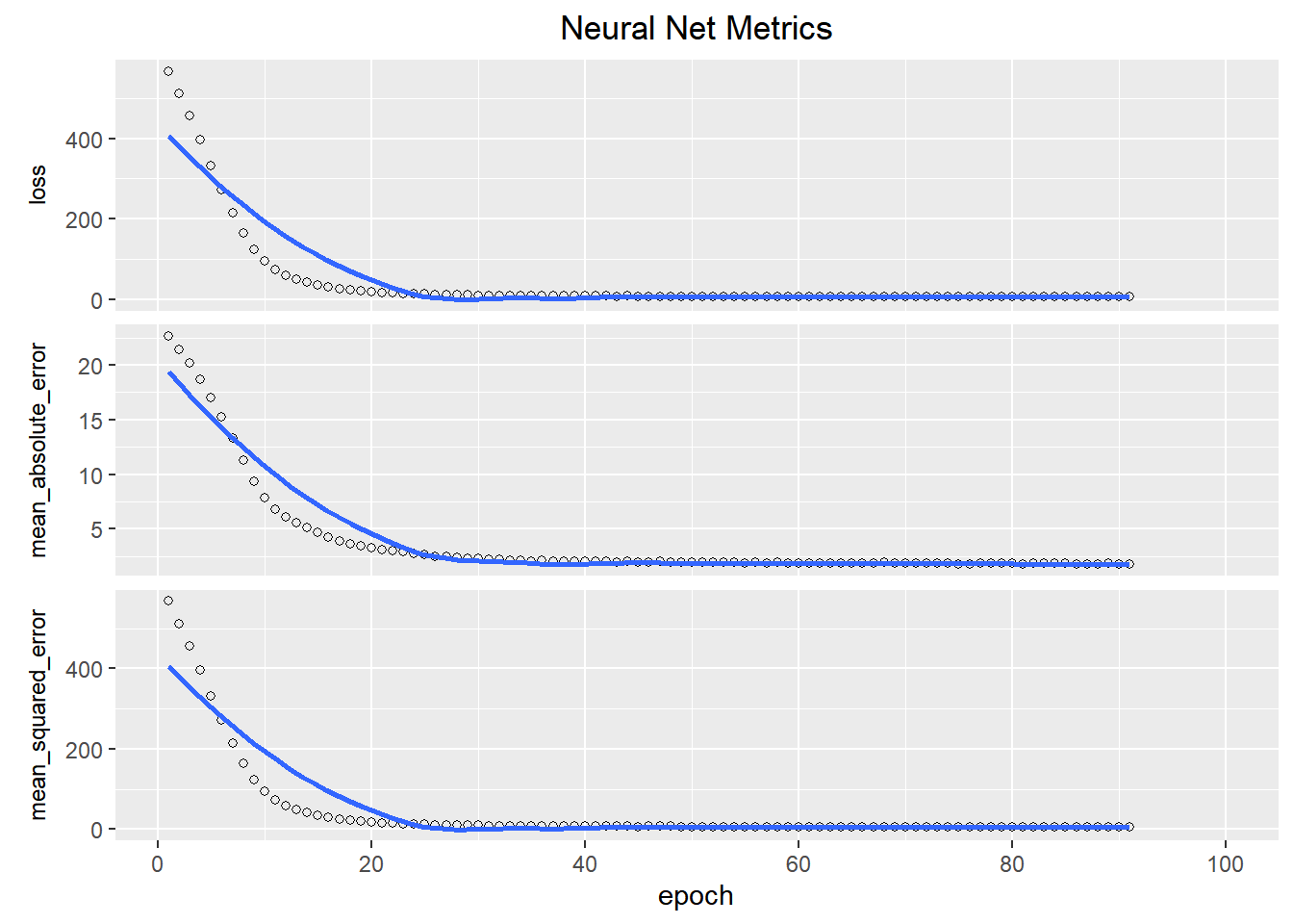
Predictions
A benefit to defining our transformation recipe is that it’s very easy to apply the same transformations to our testing data.
testing_baked = bake(rec,testing_data, composition = "matrix")
xx = subset(testing_baked, select = -MPG)
Then we just call the predict funcion. (Note that predict returns a two dimensional object, and we just want a vector to add to our dataset. That’s what the square brackets are for.)
y_pred = predict(model2, xx)[,1]Add predictions to dataset
predicted = testing_data %>%
  mutate(mpg_pred = y_pred,
         resid = MPG-mpg_pred)
Calculate some fit metrics
mae(predicted, truth = MPG, estimate = mpg_pred)
## # A tibble: 1 x 3
##   .metric .estimator .estimate
##   <chr>   <chr>          <dbl>
## 1 mae     standard        2.04
rmse(predicted, truth = MPG, estimate = mpg_pred)
## # A tibble: 1 x 3
##   .metric .estimator .estimate
##   <chr>   <chr>          <dbl>
## 1 rmse    standard        2.86
Plot the predictions
ggplot(data = predicted, aes(x = MPG))+
  geom_abline(intercept = 0, slope = 1, color = "navy")+
  geom_point(aes(y = mpg_pred))+
  coord_fixed()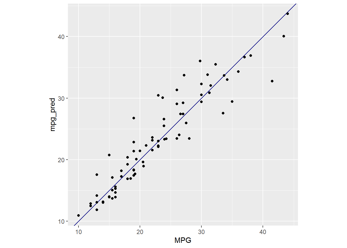
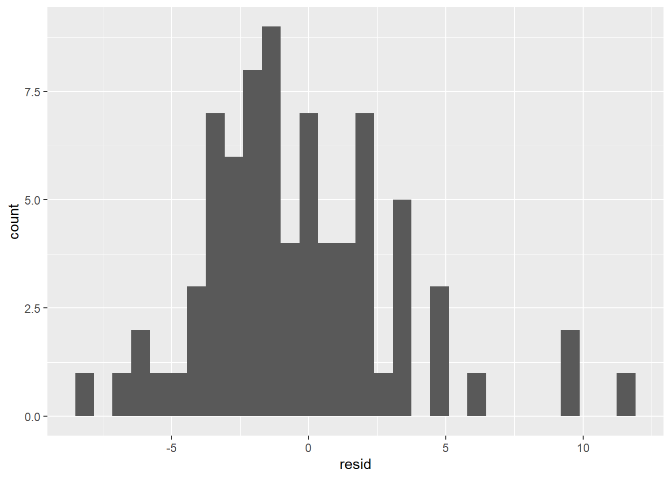
ggplot(data = predicted, aes(resid))+
  geom_histogram()
## `stat_bin()` using `bins = 30`. Pick better value with `binwidth`.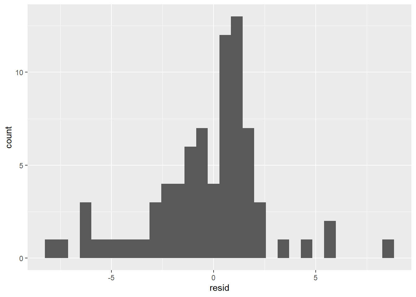
Is this better than OLS linear regression?
fit_lm = lm(MPG ~ . -1, data = training_data)
summary(fit_lm)
##
## Call:
## lm(formula = MPG ~ . - 1, data = training_data)
##
## Residuals:
##     Min      1Q  Median      3Q     Max
## -9.5117 -1.9909 -0.0752  1.8581 13.1296
##
## Coefficients:
##                Estimate Std. Error t value Pr(>|t|)
## Cylinders    -4.201e-01  3.547e-01  -1.184  0.23714
## Displacement  2.249e-02  8.230e-03   2.733  0.00664 **
## Horsepower   -2.489e-02  1.484e-02  -1.677  0.09450 .
## Weight       -6.632e-03  7.228e-04  -9.176  < 2e-16 ***
## Acceleration  4.357e-02  1.158e-01   0.376  0.70692
## `Model Year`  7.303e-01  5.684e-02  12.848  < 2e-16 ***
## USA          -1.332e+01  5.180e+00  -2.572  0.01059 *
## Europe       -1.129e+01  5.063e+00  -2.229  0.02653 *
## Japan        -1.037e+01  5.174e+00  -2.005  0.04585 *
## ---
## Signif. codes:  0 '***' 0.001 '**' 0.01 '*' 0.05 '.' 0.1 ' ' 1
##
## Residual standard error: 3.256 on 305 degrees of freedom
## Multiple R-squared:  0.9833, Adjusted R-squared:  0.9828
## F-statistic:  1991 on 9 and 305 DF,  p-value: < 2.2e-16

yy_lm = predict(fit_lm, subset(testing_data, select = -MPG))

lm_testing = testing_data %>%
  mutate(mpg_pred = yy_lm,
         resid = MPG-mpg_pred)

mae(lm_testing, truth = MPG, estimate = mpg_pred)
## # A tibble: 1 x 3
##   .metric .estimator .estimate
##   <chr>   <chr>          <dbl>
## 1 mae     standard        2.75
rmse(lm_testing, truth = MPG, estimate = mpg_pred)
## # A tibble: 1 x 3
##   .metric .estimator .estimate
##   <chr>   <chr>          <dbl>
## 1 rmse    standard        3.55
So it looks like the TensorFlow neural net performs slightly better. This may seem trivial when it comes to fitting MPG predictions based on other measurables, but in a business case, this improvement could be valuable.
ggplot(data = lm_testing, aes(x = MPG))+
  geom_abline(intercept = 0, slope = 1, color = "navy")+
  geom_point(aes(y = mpg_pred))+
  coord_fixed()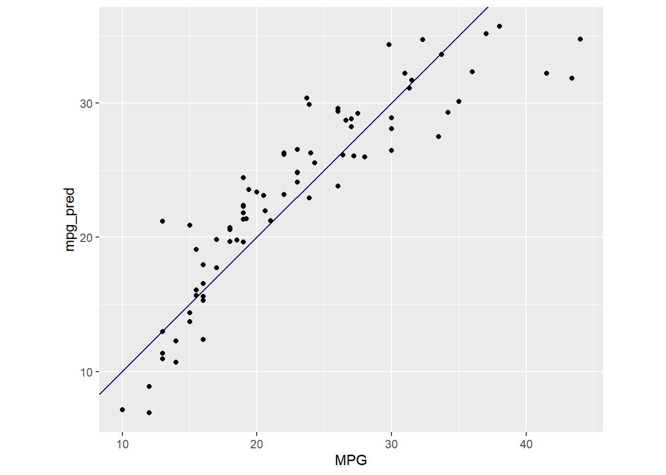
ggplot(data = lm_testing, aes(resid))+
  geom_histogram()
## `stat_bin()` using `bins = 30`. Pick better value with `binwidth`.