Intro
FiveThirtyEight has weekly riddles on The Riddler. This post is an answer to the Riddler Classic https://fivethirtyeight.com/features/how-fast-can-you-skip-to-your-favorite-song/. Here’s the gist you have a playlist of 100 songs, and when you start listening to it, you start on a random song. Your favorite song is track number 42 (thanks Douglas Adams), and every time you listen to the playlist, you try to get to track 42 as fast as possible. You listening device is no iPod, so to change songs, you only have two options.
(1) “Next,” which will take you to the next track in the list or back to song 1 if you are currently on track 100, and (2) “Random,” which will take you to a track chosen uniformly from among the 100 tracks. Pressing “Random” can restart the track you’re already listening to — this will happen 1 percent of the time you press the “Random” button.
So the question is: how quickly can you get to song 42?
Also, when a song starts playing, you instantly know what the track number is. So if song 41 starts playing, then you know that hitting the “Next” button will get you to 42.
First Thoughts
- Any time you start with a song over 42, you should hit “Random” because you would have to press “Next” all the way around 100.
- “Next” is better than “Random” at number 41 because 1 button hit gets you to 42 100% of the time, but “Random” only gets you to 42 1% of the time.
- Similarly, if you start at 40, you should just hit “Next” “Next” because “Random” “Random” is only gets you to 42 2% of the time. “Random” “Next” is only good if “Random” gets you to 41.
- There is some number between 1 and 42 that serves as the turning point between “Next” and “Random.”
- Figuring out that number using probabilities and expectations using algebra seems harder than just simulating the results.
Answer
I can get to 42 in 12.5 steps, on average. Here’s my strategic thought process and how I got to the number.
Simulation in R
I’m going to walk through my thought process around coding this up. I hope this is a bit more illuminating than just jumping ahead to my final answer.
Setup
Load the tidyverse
library(tidyverse)
## -- Attaching packages ------------------- tidyverse 1.3.0 --
## v ggplot2 3.2.1     v purrr   0.3.3
## v tibble  2.1.3     v dplyr   0.8.3
## v tidyr   1.0.0     v stringr 1.4.0
## v readr   1.3.1     v forcats 0.4.0
## -- Conflicts ---------------------- tidyverse_conflicts() --
## x dplyr::filter() masks stats::filter()
## x dplyr::lag()    masks stats::lag()
Code in the functions
“Next” track adds 1 to the supplied number unless the supplied number is 100, in which case it returns to the first track.
The only difference here for coding “Random” using R instead of a different programming language is that you have to frame the random number generator in R using the uniform distribution.
next_track = function(i){
  if(i == 100) {
    return (1)
  } else {
  return(i+1)
  }
}

random_track = function(){
  return(round(runif(n = 1, min = 1, max = 100)))
}
Find the expected number of button presses if you use 21 as the cutoff for “Next” vs “Random”
There’s a decent amount going on in this next code chunk:
tests_to_repeat = 1000

long_term = NULL

    for (i in 1:tests_to_repeat) {

      # Initialize starting variables

      track_position = random_track()
      button_presses = 0

      while (track_position != 42) {
        if  (track_position <= 41 &  track_position >= 21) {
          button_presses = button_presses + 1
          track_position = next_track(track_position)
        } else {
          button_presses = button_presses + 1
          track_position = random_track()
        }
      }

      long_term = c(long_term, button_presses)
    }
We’re going to run 1,000 simulations of this, and we’re going to use long_term to track the number of botton presses over the long term.
Inside the for-loop, we will record the track position (starting with a random track) and the number of button presses.
The while-loop runs until we get to track 42. If we’re between 41 and 21 (inclusively), then we hit the “Next” button. If we’re outside of that range, then we take our chances with “Random” and repeat as necessary.
This plot shows the results of our simulations.
plot(long_term, xlab = "Simulation Index", ylab = "Button Presses")
abline(h = mean(long_term))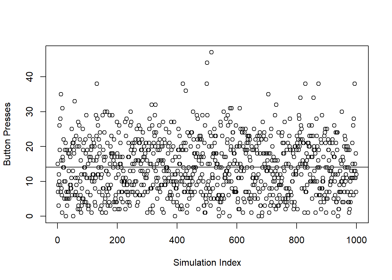
mean(long_term)
## [1] 14.045
So it takes just over 14 button presses, on average, to get to 42 if your strategy is to “Random” into the range of 21 to 41, and then hit “Next.”
Is 21 the best cutoff?
So we could brute-force the simulations and go one-by-one increasing the cutoff until we get increasing means, or we can loop through the iterations. The only thing is, this type of thing can take a little while, so I decided to leverage my computers multiple cores.
Parallel Computing in R
My laptop has four cores, but with desktops, cloud options, and servers, you can get a lot more horsepower. I’m going to use the doSNOW and foreach packages.
# library(tidyverse)
library(doSNOW)
## Loading required package: foreach
##
## Attaching package: 'foreach'
## The following objects are masked from 'package:purrr':
##
##     accumulate, when
## Loading required package: iterators
## Loading required package: snow
library(foreach)
Create clusters
The way these packages handle parallel computing is to create clusters that can initiate an R script. Each cluster then uses a core to run the code. This is the standard way to initialize and register the number of clusters. I’m going to create three clusters to use three of four cores, so hopefully, my laptop will still be useable while this runs.
cl<-makeCluster(3) # change the 2 to the number of CPU cores you want to use
registerDoSNOW(cl)
Foreach loop
Instead of a for-loop, we’re going to write a foreach-loop. Here’s where I read about the basics of foreach https://www.r-bloggers.com/parallel-r-loops-for-windows-and-linux/.
foreach usually results in a list, but we can get it to output a dataframe by adding .combine = 'rbind'. %dopar% is the parallel version of %do%, and the only thing different is that it requires preregistered clusters.
I shouldn’t brush aside that I’m actually recording means instead of all the tests. However, means are consistent, so the mean button presses for a strategy converges on the same number as the mean of test means. So tests_to_repeat is the same as above, and means_to_capture is the number of times I’m going to repeat the code above.
# Initialize starting variables

tests_to_repeat = 1000
means_to_capture = 1000

mean_tests = foreach(j=1:41, .combine = 'rbind') %dopar% {

  means = NULL

  for (k in 1:means_to_capture) {

    long_term = NULL

    for (i in 1:tests_to_repeat) {

      track_position = random_track()
      button_presses = 0

      while (track_position != 42) {
        if  (track_position <= 41 &  track_position >= j) {
          button_presses = button_presses + 1
          track_position = next_track(track_position)
        } else {
          button_presses = button_presses + 1
          track_position = random_track()
        }
      }

      long_term = c(long_term, button_presses)
    }

    means = vctrs::vec_rbind(means, tibble::tibble(test_iter = k,
                                                   low_cutoff = j,
                                                   mean_steps = mean(long_term)))

  }

  means

}
Instead of using return(variable), foreach-loops just need you to type the variable name you want to return.
Stop clusters
Now we’ll close our clusters. Eventually, the clusters close after some period of inactivity, but it’s best practice to stop them in the code.
stopCluster(cl)Results
Here’s a plot of the final mean_tests results.
ggplot(data = mean_tests, aes(x = low_cutoff, y = mean_steps))+
geom_point(aes(color = test_iter))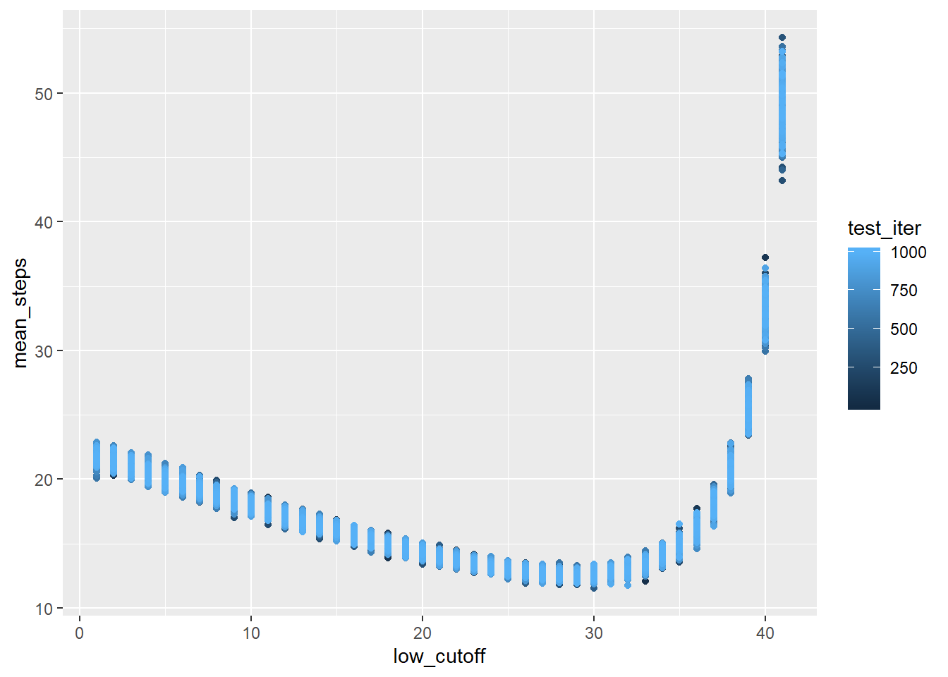 It looks like using a cutoff between 26 and 31 results in the fewest number of button presses, but it’s tough to see in the scatter plot. The means are pretty tightly grouped already, but a boxplot will show a bit more detail. I’m also going to trim off some of the worse strategies.
filtered_simulations = mean_tests %>%
  filter(low_cutoff <= 33,
         low_cutoff >= 23)

ggplot(data = filtered_simulations, aes(x = low_cutoff, y = mean_steps))+
  geom_boxplot(aes(group = low_cutoff))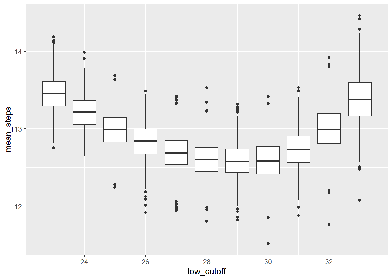
Okay, so 29 appears to be the preferred cutoff. But it’s not much better than some of the other cutoffs around it.
filtered_simulations %>%
  group_by(low_cutoff) %>%
  summarize(avg_steps = mean(mean_steps)) %>%
  arrange(avg_steps) %>%
  kableExtra::kable(align = 'c') %>%
  kableExtra::kable_styling("striped", full_width = FALSE) %>%
kableExtra::add_header_above(c("Sorted Results" = 2))| low_cutoff | avg_steps |
|---|---|
| 29 | 12.58122 |
| 30 | 12.59304 |
| 28 | 12.60666 |
| 27 | 12.69308 |
| 31 | 12.73427 |
| 26 | 12.83574 |
| 25 | 12.99733 |
| 32 | 13.00494 |
| 24 | 13.21565 |
| 33 | 13.38531 |
| 23 | 13.45534 |
To really prove this out, it would be better to run more simulations and also prove it algebraically. I may try to tackle the algebraic proof in another post, but no guarantees. I’m pretty sure you’d have to write out the expected number of button presses for different strategies.